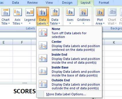
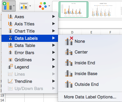
41 excel chart hide zero labels

Display or hide zero values - support.microsoft.com Select the cells with hidden zeros. You can press Ctrl+1, or on the Home tab, click Format > Format Cells. Click Number > General to apply the default number format, and then click OK. Hide zero values returned by a formula Select the cell that contains the zero (0) value. How to hide zero in chart axis in Excel? - ExtendOffice 1. Right click at the axis you want to hide zero, and select Format Axis from the context menu. 2. In Format Axis dialog, click Number in left pane, and select Custom from Category list box, then type #"" in to Format Code text box, then click Add to add this code into Type list box. See screenshot:

Automatically eliminating zero-value data labels from charts Automatically eliminating zero-value data labels from charts. I have a pie chart drawn from the following data: Item A: 10. Item B: 0 (in place as I might expect some value at a later time) Item C: 30. Item D: 60. I did away with the legend in favor of data labels on each slice of the pie, showing percentages. So Excel generates:

Excel chart hide zero labels

Radar chart hide null and zero values categories - Microsoft Community However, I found a workaround that is to transpose (rotate) data from rows to columns or vice versa first (or recreate the table manually), then insert a chart and a filter for the new table, when you untick "0", the categories labels containing "0" will be hidden. Hope it can be helpful to you, if you have any concerns please feel free ... How can I hide 0-value data labels in an Excel Chart? How can I hide 0-value data labels in an Excel Chart? Right click on a label and select Format Data Labels. Go to Number and select Custom. Enter #"" as the custom number format. Repeat for the other series labels. Zeros will now format as blank. NOTE This answer is based on Excel 2010, but should work in all versions Hide category names from pie chart if value is zero - MrExcel Message Board I have a pie chart in Excel 2010 where I need to show category name, percentage and leader lines in the chart. The data typically have some zero values in it that I do not want to show on the pie chart. I can hide the zero percentages by using custom number format 0,0 %;-0,0 %;"" but it still leaves the category name and the leader lines ...

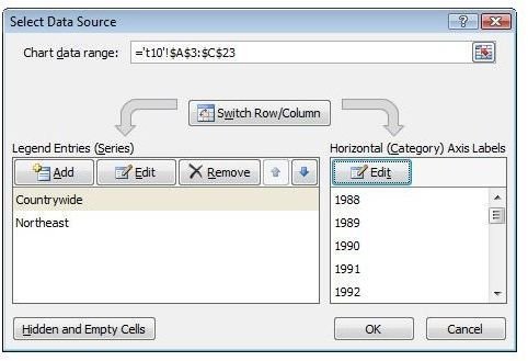
Excel chart hide zero labels. Hiding data labels with zero values | MrExcel Message Board Right click on a data label on the chart (which should select all of them in the series), select Format Data Labels, Number, Custom, then enter 0;;; in the Format Code box and click on Add. If your labels are percentages, enter 0%;;; or whatever format you want, with ;;; after it. With stacked column charts, you have to do this for each series ... Hide legend items in a graph when associated value = zero or blank 6. right-click your chart & Select Data. Edit the Legend Entries. change the series values to show the sheet name, exclamation mark & your Named Range for FTP. so mine looks like this: =Charts!FTP also in screenshot inside file 7. similarly, right-click your chart & Select Data. Edit the Horizontal Axis. How to eliminate zero value labels in a pie chart - MrExcel Message Board However you can hide the 0% using custom number formatting. Right click the label and select Format Data Labels. Then select the Number tab and then Custom from the Categories. Enter. 0%; [White] [=0]General;General. in the Type box. This will set the font colour to white if a label has a value of zero. Hide zero value data labels for excel charts (with category name) Hide zero value data labels for excel charts (with category name) I'm trying to hide data labels for an excel chart if the value for a category is zero. I already formatted it with a custom data label format with #%;;; As you can see the data label for C4 and C5 is still visible, but I just need the category name if there is a value.

How to hide zero data labels in chart in Excel? - ExtendOffice In the Format Data Labelsdialog, Click Numberin left pane, then selectCustom from the Categorylist box, and type #""into the Format Codetext box, and click Addbutton to add it to Typelist box. See screenshot: 3. Click Closebutton to close the dialog. Then you can see all zero data labels are hidden. How to suppress 0 values in an Excel chart | TechRepublic You can hide the 0s by unchecking the worksheet display option called Show a zero in cells that have zero value. Here's how: Click the File tab and choose Options. In Excel 2007, click the Office... Hide data labels with low values in a chart - Excel Help Forum Hide data labels with low values in a chart. To hide chart data labels with zero value I can use the custom format 0%;;;, But is there also a possibility to hide data labels in a chart with values lower that a certain predefined number (e.g. hide all labels < 2%)? Register To Reply. 03-29-2013, 12:06 PM #2. Andy Pope. Remove Zeros from chart labels - Online Excel Training Occasionally you have a chart where the data is blank, but on the chart you see zeros for the labels as shown below. One way to get rid of this is to create a custom format for the numbers where a zero is shown with a blank. To see the full course contents click here. Previous Next 0 Continue Shopping

Hide data labels with zero values WITHOUT changing number format How to hide data labels with zero value? I did a bit search but all solutions suggested are by changing number format. As I already have a defined number format in the chart, changing format is not an option. Also, VBA is not an option. Excel Facts Format cells as date Click here to reveal answer 1 2 Next Michael M Well-known Member Joined How can I hide 0-value data labels in an Excel Chart? Right click on a label and select Format Data Labels. Go to Number and select Custom. Enter #"" as the custom number format. Repeat for the other series labels. Zeros will now format as blank. NOTE This answer is based on Excel 2010, but should work in all versions Share Improve this answer edited Jun 12, 2020 at 13:48 Community Bot 1 How to hide points on the chart axis - Microsoft Excel 2016 This tip will show you how to hide specific points on the chart axis using a custom label format. To hide some points in the Excel 2016 chart axis, do the following: 1. Right-click in the axis and choose Format Axis... in the popup menu: 2. On the Format Axis task pane, in the Number group, select Custom category and then change the field ... Pie Chart - Remove Zero Value Labels - Excel Help Forum The formulas in the source table can be written in such a way as to mask the zero or error values, but they still show up in the chart. Solution (Tested in Excel 2010.): 1. Right click on one of the chart "data labels" and choose "Format Data Labels." 2. Choose "Number" from the vertical menu on the left. 3.

how to make a excel graph.

How can I hide 0% value in data labels in an Excel Bar Chart The quick and easy way to accomplish this is to custom format your data label. Select a data label. Right click and select Format Data Labels; Choose the Number category in the Format Data Labels dialog box.

How to Change Labels for a Chart Axis in Excel 2007

How to Quickly Remove Zero Data Labels in Excel - Medium In this article, I will walk through a quick and nifty "hack" in Excel to remove the unwanted labels in your data sets and visualizations without having to click on each one and delete manually....

How to Make Charts and Graphs in Excel | Smartsheet

Hide Series Data Label if Value is Zero - Peltier Tech Then apply custom number formats to show only the appropriate labels. In Number Formats in Excel I show how the number format provides formats for positive, negative, and zero values, and for text, with the individual formats separated by semicolons: ;;; Apply the following three number formats to the three sets of value data labels:

Contoh Yes No Question - Hosof

Hide 0-value data labels in an Excel Chart - Exceltips.nl Browse: Home / Hide 0-value data labels in an Excel Chart 1) Right click on a label and select Format Data Labels. 2) Go to Number and select Custom. 3) Enter #"" as the custom number format. 4) Repeat for the other series labels. 5) Zeros will now format as blank « Get month from weeknumber Set all Pivot values to SUM and correct FORMAT »

Lesson 2 | How to Create Charts Using Microsoft Excel Tutorial

Hide zero values in chart labels- Excel charts WITHOUT zeros ... - YouTube 00:00 Stop zeros from showing in chart labels00:32 Trick to hiding the zeros from chart labels (only non zeros will appear as a label)00:50 Change the number...

One click to add total label to stacked chart in Excel

I do not want to show data in chart that is "0" (zero) If your data doesn't have filters, you can switch them on by clicking Data > Sort & Filter > Filter on the Excel Ribbon. You can filter out the zero values by unchecking the box next to 0 in the filter drop-down. After you click OK all of the zero values disappear (although you can always bring them back using the same filter).

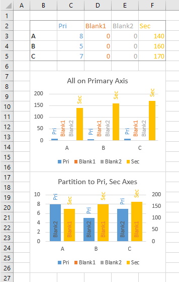
Excel Column Chart with Primary and Secondary Axes - Peltier Tech Blog

Hide category names from pie chart if value is zero - MrExcel Message Board I have a pie chart in Excel 2010 where I need to show category name, percentage and leader lines in the chart. The data typically have some zero values in it that I do not want to show on the pie chart. I can hide the zero percentages by using custom number format 0,0 %;-0,0 %;"" but it still leaves the category name and the leader lines ...

Share :