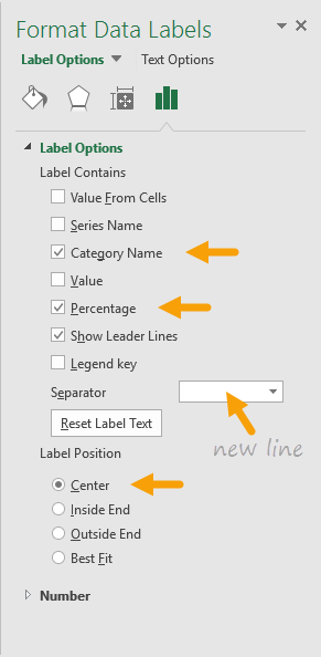
41 how to add percentage and category name data labels in excel

How to use Excel Data Model & Relationships - Chandoo.org Jul 01, 2013 · Handling large volumes of data in Excel—Since Excel 2013, the “Data Model” feature in Excel has provided support for larger volumes of data than the 1M row limit per worksheet. Data Model also embraces the Tables, Columns, Relationships representation as first-class objects, as well as delivering pre-built commonly used business scenarios ... Excel charts: add title, customize chart axis, legend and data labels Depending on where you want to focus your users' attention, you can add labels to one data series, all the series, or individual data points. Click the data series you want to label. To add a label to one data point, click that data point after selecting the series. Click the Chart Elements button, and select the Data Labels option.

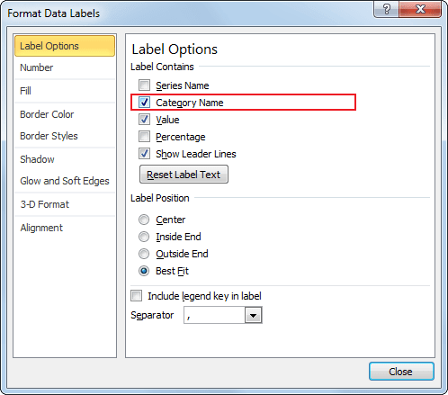
How to show data label in "percentage" instead of - Microsoft Community If so, right click one of the sections of the bars (should select that color across bar chart) Select Format Data Labels Select Number in the left column Select Percentage in the popup options In the Format code field set the number of decimal places required and click Add.

How to add percentage and category name data labels in excel

Solved: change data label to percentage - Power BI 1 ACCEPTED SOLUTION az38 Super User 06-08-2020 11:22 AM Hi @MARCreading pick your column in the Right pane, go to Column tools Ribbon and press Percentage button do not hesitate to give a kudo to useful posts and mark solutions as solution LinkedIn View solution in original post Message 2 of 7 1,631 Views 1 Reply All forum topics Previous Topic Format Number Options for Chart Data Labels in Excel 2011 ... - Indezine Figure 1: Chart with Data Values added as Data Labels. Follow these steps to learn how to format the values used in Data Labels within Excel 2011: Select the chart -- then select the Charts tab which appears on the Ribbon, as shown highlighted in red within Figure 2. Within the Charts tab, click the Edit button (highlighted in blue within ... Solve Equation in Excel | How to Solve Equation with Solver ... Goal Seek: It is an inbuilt function in excel under What-If Analysis, which helps us solve equations to source cell values until the desired output is achieved. Recommended Articles. This is a guide to Solve Equation in Excel. Here we discuss how to add the Solver Add-in Tool and how to Solve equations with Solver Add-in Tool in excel.

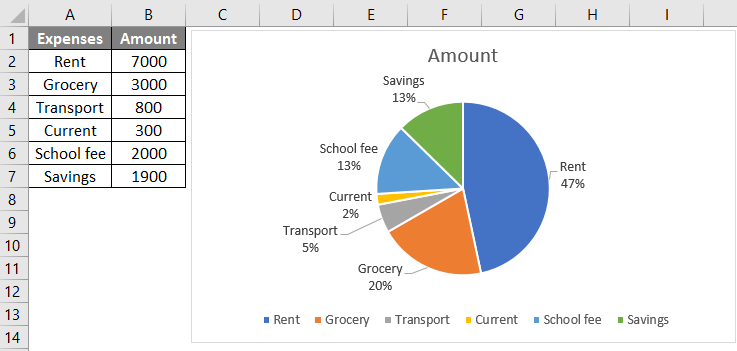
How to add percentage and category name data labels in excel. How to Change Excel Chart Data Labels to Custom Values? First add data labels to the chart (Layout Ribbon > Data Labels) Define the new data label values in a bunch of cells, like this: Now, click on any data label. This will select "all" data labels. Now click once again. At this point excel will select only one data label. How To Add and Remove Legends In Excel Chart? - EDUCBA If we want to add the legend in the excel chart, it is a quite similar way how we remove the legend in the same way. Select the chart and click on the “+” symbol at the top right corner. From the pop-up menu, give a tick mark to the Legend. How to add data labels from different column in an Excel chart? Right click the data series in the chart, and select Add Data Labels > Add Data Labels from the context menu to add data labels. 2. Click any data label to select all data labels, and then click the specified data label to select it only in the chart. 3. How to Add Percentage Axis to Chart in Excel To do this, we will select the whole table again, and then go to Insert >> Charts >> 2-D Columns: To show percentages on a second axis, we first need to click anywhere on the orange bars that we have on our graph (this is not easy in this example as they are rather small). Once we do, we will right-click on it, and then select Format Data Series:

Apply Custom Data Labels to Charted Points - Peltier Tech Double click on the label to highlight the text of the label, or just click once to insert the cursor into the existing text. Type the text you want to display in the label, and press the Enter key. Repeat for all of your custom data labels. This could get tedious, and you run the risk of typing the wrong text for the wrong label (I initially ... Best Types of Charts in Excel for Data Analysis, Presentation ... Apr 29, 2022 · Use the moving average trendline if there is a lot of fluctuation in your data. How to add a chart to an Excel spreadsheet? To add a chart to an Excel spreadsheet, follow the steps below: Step-1: Open MS Excel and navigate to the spreadsheet, which contains the data table you want to use for creating a chart. Step-2: Select data for the chart: How to show percentages in stacked column chart in Excel? Add percentages in stacked column chart 1. Select data range you need and click Insert > Column > Stacked Column. See screenshot: 2. Click at the column and then click Design > Switch Row/Column. 3. In Excel 2007, click Layout > Data Labels > Center . In Excel 2013 or the new version, click Design > Add Chart Element > Data Labels > Center. 4. Custom Chart Data Labels In Excel With Formulas Follow the steps below to create the custom data labels. Select the chart label you want to change. In the formula-bar hit = (equals), select the cell reference containing your chart label's data. In this case, the first label is in cell E2. Finally, repeat for all your chart laebls.

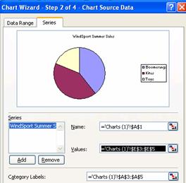
How to Add Data Labels to an Excel 2010 Chart - dummies Use the following steps to add data labels to series in a chart: Click anywhere on the chart that you want to modify. On the Chart Tools Layout tab, click the Data Labels button in the Labels group. A menu of data label placement options appears: None: The default choice; it means you don't want to display data labels. Understanding Excel Chart Data Series, Data Points, and Data Labels Select a data series in a column chart. All columns of the same color are highlighted. Each column is surrounded by a border that includes small dots on the corners. Select the column in the chart to be modified. Only that column is highlighted. Select the Format tab. Add a DATA LABEL to ONE POINT on a chart in Excel Steps shown in the video above: Click on the chart line to add the data point to. All the data points will be highlighted. Click again on the single point that you want to add a data label to. Right-click and select ' Add data label ' This is the key step! Right-click again on the data point itself (not the label) and select ' Format data label '. excel - How can I add chart data labels with percentage? - Stack Overflow I want to add chart data labels with percentage by default with Excel VBA. Here is my code for creating the chart: Private Sub CommandButton2_Click () ActiveSheet.Shapes.AddChart.Select ActiveChart.SetSourceData Source:=Range ("'Sheet1'!$A$6:$D$6") ActiveChart.ChartType = xlDoughnut End Sub It only creates Doughnut chart with no information labels.

Pie Chart Examples | Types of Pie Charts in Excel with Examples

Excel tutorial: How to use data labels Generally, the easiest way to show data labels to use the chart elements menu. When you check the box, you'll see data labels appear in the chart. If you have more than one data series, you can select a series first, then turn on data labels for that series only. You can even select a single bar, and show just one data label.

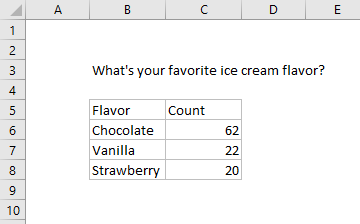
Pie Chart: Survey results favorite ice cream flavor | Exceljet

Count and Percentage in a Column Chart - ListenData Download the workbook. Steps to show Values and Percentage. 1. Select values placed in range B3:C6 and Insert a 2D Clustered Column Chart (Go to Insert Tab >> Column >> 2D Clustered Column Chart). See the image below. Insert 2D Clustered Column Chart. 2. In cell E3, type =C3*1.15 and paste the formula down till E6.

CD: Pie Charts

Multiple Data Labels on bar chart? - Excel Help Forum looks like you are not changing the data labels settings from show Value to show category labels. Apply data labels to series 1 inside end Select A1:D4 and insert a bar chart Select 2 series and delete it Select 2 series, % diff base line, and move to secondary axis Adjust series 2 data references, Value from B2:D2 Category labels from B4:D4

Set up PivotTables using the PowerPivot add-on module

Add data labels and callouts to charts in Excel 365 - EasyTweaks.com Step #2: When you select the "Add Labels" option, all the different portions of the chart will automatically take on the corresponding values in the table that you used to generate the chart. The values in your chat labels are dynamic and will automatically change when the source value in the table changes. Step #3: Format the data labels.

Pie Chart: Survey results favorite ice cream flavor | Exceljet

How to Add Data Bars in Excel? - EDUCBA Follow the below steps to add data bars in Excel. Step 3: Select the number range from B2 to B11. Step 4: Go to the HOME tab. Select Conditional Formatting and then select Data Bars. Here we have two different categories to highlight; select the first one. Step 5: Now, we have a beautiful bar inside the cells.

Excel Is Fun

Multiple data labels (in separate locations on chart) Running Excel 2010 2D pie chart I currently have a pie chart that has one data label already set. The Pie chart has the name of the category and value as data labels on the outside of the graph. I now need to add the percentage of the section on the INSIDE of the graph, centered within the pie section.

Excel 3-D Pie charts - Microsoft Excel 2016

Video: Customize a pie chart - support.microsoft.com In the labels, the dollar amounts are replaced with percentages. I’d also like to show the Salesperson’s name. So, in the pane, I’ll check Category Name. A name and percentage now show in the data label. I’ll click X to close the pane. I like the labels, though the ones at the top are crowded under the title. To fix that, I can rotate ...

Excel 3-D Pie charts - Microsoft Excel 2010

Add or remove data labels in a chart - support.microsoft.com Add data labels to a chart Click the data series or chart. To label one data point, after clicking the series, click that data point. In the upper right corner, next to the chart, click Add Chart Element > Data Labels. To change the location, click the arrow, and choose an option.